Ok fasting hours, but how about eating hours?
The data dump from my Zero fasting app highlights the fasting hours. I had used Zero from 2019 to late 2023, and I wanted to look at briefly, well what about the eating hours, other than the fasted hours?
In an effort to save time, I used ChatGPT to come up with the calculation around the eating hours. Actually the first try was interesting since the outcome was showing daily eating hours that were beyond 40 hours 😅, but coercing ChatGPT to try to correct so this falls within the expected under 10 hours, ChatGPT was able to actually course correct nicely ! Impressed.
In any case, here is some final stage analysis, with my own updates/cleanup, to get this running locally.
from pathlib import Path
import pandas as pd
import pylab
import matplotlib.pyplot as plt

from datetime import datetime
import pytz
import pandas as pd

def utc_ts():
    utc_now = datetime.utcnow().replace(tzinfo=pytz.UTC)
    return utc_now.strftime('%Y-%m-%dT%H%M%S')

data = pd.read_csv("2024-06-02-Updated_Zero_Fast_Data.csv")


data["start_timestamp"] = pd.to_datetime(data["start_timestamp"])
data["end_timestamp"] = pd.to_datetime(data["end_timestamp"])


data["year"] = data["start_timestamp"].map(lambda x:x.year)

# Sort the dataset by start_timestamp
data_sorted = data.sort_values(by='start_timestamp').reset_index(drop=True)

# Recalculate eating_hours with the sorted dataset
eating_hours_list_sorted = []
for i in range(len(data_sorted) - 1):
    next_start_timestamp = data_sorted.at[i + 1, 'start_timestamp']
    end_timestamp = data_sorted.at[i, 'end_timestamp']
    eating_hours = abs((next_start_timestamp - end_timestamp).total_seconds() / 3600)
    eating_hours_list_sorted.append(eating_hours)

# Add NaN for the last row
eating_hours_list_sorted.append(pd.NA)

# Update the sorted dataframe
data_sorted['eating_hours'] = eating_hours_list_sorted

# Display the first few rows of the sorted and updated dataframe
data_sorted[['start_timestamp',  'end_timestamp', 'eating_hours']].head(20)


data_sorted['eating_hours'] = pd.to_numeric(data_sorted['eating_hours'], errors='coerce')


# Calculate the 7-day rolling average for eating_hours
data_sorted['rolling_avg_eating_hours'] = data_sorted['eating_hours'].rolling(window=7).mean()

# Plot the 7-day rolling average of eating_hours against start_timestamp
plt.figure(figsize=(12, 6))
plt.plot(data_sorted['start_timestamp'], data_sorted['rolling_avg_eating_hours'], marker='o', linestyle='-', color='b')
plt.xlabel('Date')
plt.ylabel('7-Day Rolling Average Eating Hours')
plt.title('7-Day Rolling Average of Eating Hours vs Date')
plt.grid(True)
plt.xticks(rotation=45)
plt.tight_layout()

# Display the plot


out_loc = f"{utc_ts()}-plot.png"
pylab.savefig(out_loc)
pylab.close()
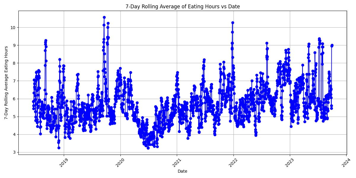
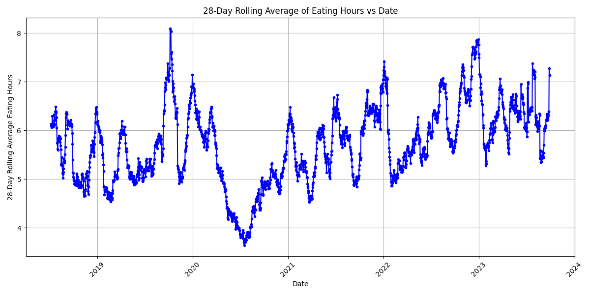
So the 7 day rolling average was too tight, so I tried 28 day instead.
plt.figure(figsize=(12, 6))
plt.plot(data_sorted['start_timestamp'], data_sorted['rolling_avg_eating_hours'], marker='.', linestyle='-', color='b')
plt.xlabel('Date')
plt.ylabel('28-Day Rolling Average Eating Hours')
plt.title('28-Day Rolling Average of Eating Hours vs Date')
plt.grid(True)
plt.xticks(rotation=45)
plt.tight_layout()

# Display the plot


out_loc = f"{utc_ts()}-plot.png"
pylab.savefig(out_loc)
pylab.close()
And let’s use a histogram overlay for comparisons year over year
So at some point, I started eating earlier in the day after the stricter fasts. Let’s look at this data now slightly differently. (I didn’t bother with ChatGPT at this point since the analysis was running into some errors and plotting was no longer working, so just went manual.)
comparisons = [[2019, 2020], [2020, 2021], [2021, 2022], [2022, 2023]]

fig, axes = plt.subplots(figsize=(12,6), nrows=len(comparisons), ncols=1)
fig.patch.set_facecolor("xkcd:mint green")
plt.tight_layout()
for i, (year1, year2) in enumerate(comparisons):

    df1 = data_sorted[data_sorted["year"] == year1]
    df2 = data_sorted[data_sorted["year"] == year2]

    # menusdf[col + "_num_tokens"] = menusdf[col].map(lambda x: len(x.split(" "))) #  if isinstance(x, str) else 0
    ax = axes[i]
    ax.hist(df1["eating_hours"], bins=50, alpha=0.2, color="r", density=True)
    ax.hist(df2["eating_hours"], bins=50, alpha=0.2, color="b", density=True)
    ax.set(title=f"compare {year1}(red) to {year2}(blue)")

out_loc = f"{utc_ts()}-plot.png"
pylab.savefig(out_loc)
pylab.close()
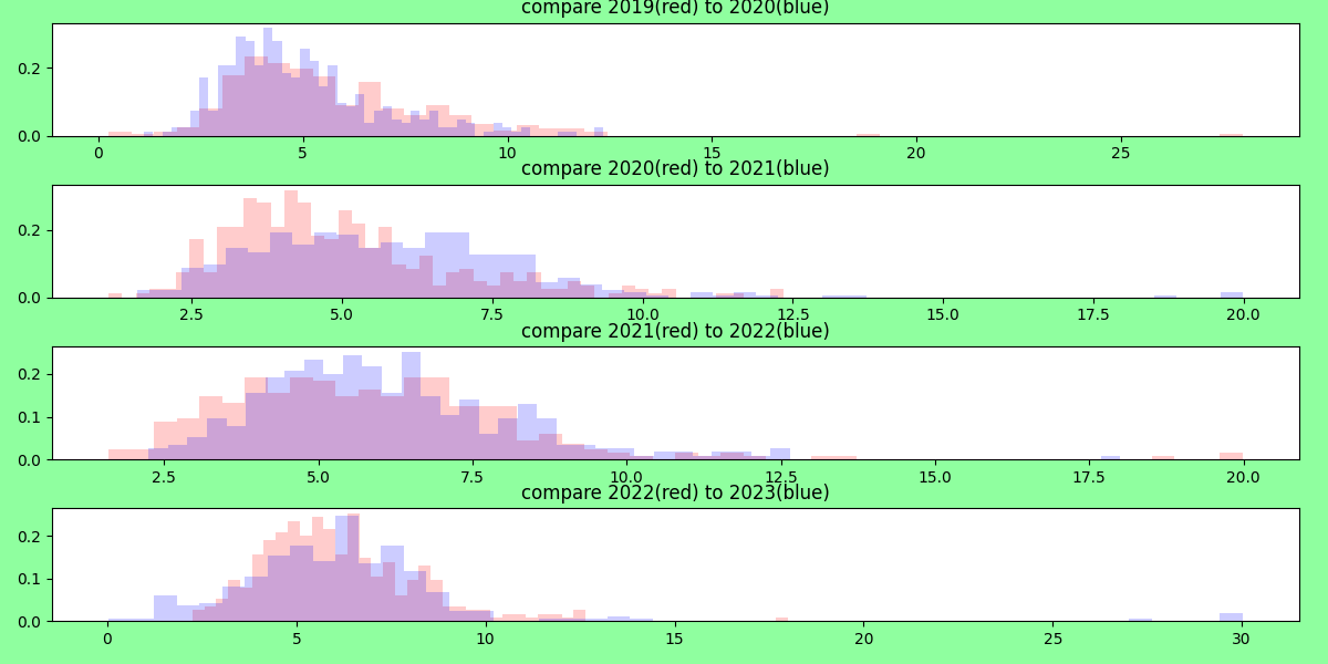
Ok I can tell for almost each year over year comparison, the number of eating hours slightly increases.
All this sparked per discussing fasting with a friend
A friend had recently reached the 48 hour mark of a fast and I started reflecting also. I dug up this one time I tried a longer restriction too,

Ultimately I think I prefer, as the main character in Blade Runner 2044 says, to "… keep an empty stomach until the difficult part of the day is done." This feel right. Beyond that, I realize this creates some later-day-eating-anti-patterns.
I know that clinical data (not citing here because I don’t recall the exact finding), has found that eating slight earlier, is associated with a lower likelihood of overconsumption of calories. That is where my mind is heading to next 🧐.