• [[my backprop SGD from scratch 2022-Aug]]
    • 13:16 so per yesterday, wondering why is it that the network I have is producing basically the same result , around 0.48 for any inputs. And that's true both in my original matrix-multiplication code and manually constructed too.
      • So lets say for a simple network, y_prob = sigmoid(x1*w1 + x2*w2) where x1 and x2 are also outputs of sigmoids, in (0, 1) , what are possible values for y_prob ?


        			  import numpy as np 
        			  from itertools import product
        			  import pylab
        			  import matplotlib.pyplot as plt
        			  
        			  from utils import utc_now, utc_ts
        			  import plot
        			  
        			  side = 5
        			  vec = []
        			  for i in range(side*side):
        			  	w1, w2 = -0.5 + np.random.random((2, ))
        			  	vec.append(
        			        	[
        			  		    [
        			  			  	n.logit_to_prob(x1*w1 + x2*w2) 
        			  				for x1, x2 in product(np.arange(0, 1, .01), np.arange(0, 1, .01))
        			              ],
        			      		f"w1={round(w1, 2)}, w2={round(w2, 2)}"	
        			      	])
        			      
        			  out_loc = plot.plot_grid(vec, side=5, title="y_prob-outputs")
        			      
        			  
        			  # saving to 2022-10-13T185339-y_prob-outputs.png
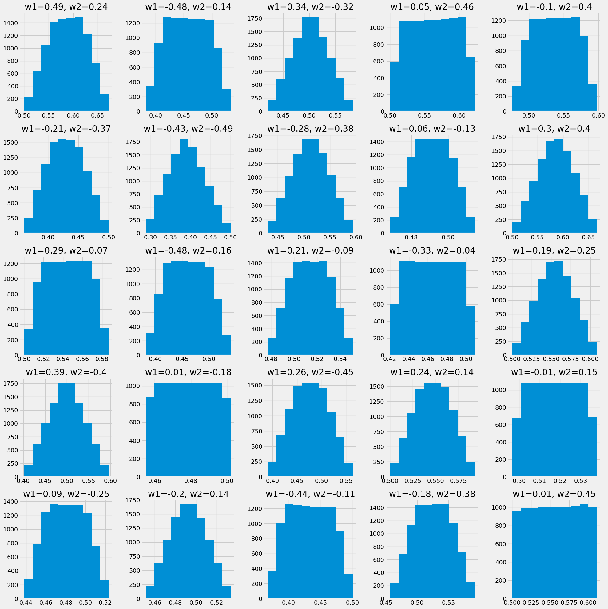


      • ok so yea we have a pretty tight range just from this. Hmm let me see what happens if I were to add a bunch of extra nodes.


        			  side = 5
        			  vec = []
        			  for i in range(side*side):
        			  	w1, w2, w3, w4, w5 = -0.5 + np.random.random((5, ))
        			  	vec.append(
        			        	[
        			  		    [
        			  			  	n.logit_to_prob(x1*w1 + x2*w2 + x3*w3 + x4*w4 + x5*w5) 
        			  				for x1, x2, x3, x4, x5 in product(
        			                    np.arange(0, 1, .1), 
        			                    np.arange(0, 1, .1), 
        			                    np.arange(0, 1, .1), 
        			                    np.arange(0, 1, .1), 
        			                    np.arange(0, 1, .1)
        			                  )
        			              ],
        			              
        			      		f"w1={round(w1, 1)}, w2={round(w2, 1)}, w3={round(w3, 1)}, w4={round(w4, 1)}, w5={round(w5, 1)}"	
        			      	])
        			      
        			  out_loc = plot.plot_grid(vec, side=5, title="y_prob-outputs")
        			  
        			  # saving to 2022-10-13T200559-y_prob-outputs.png
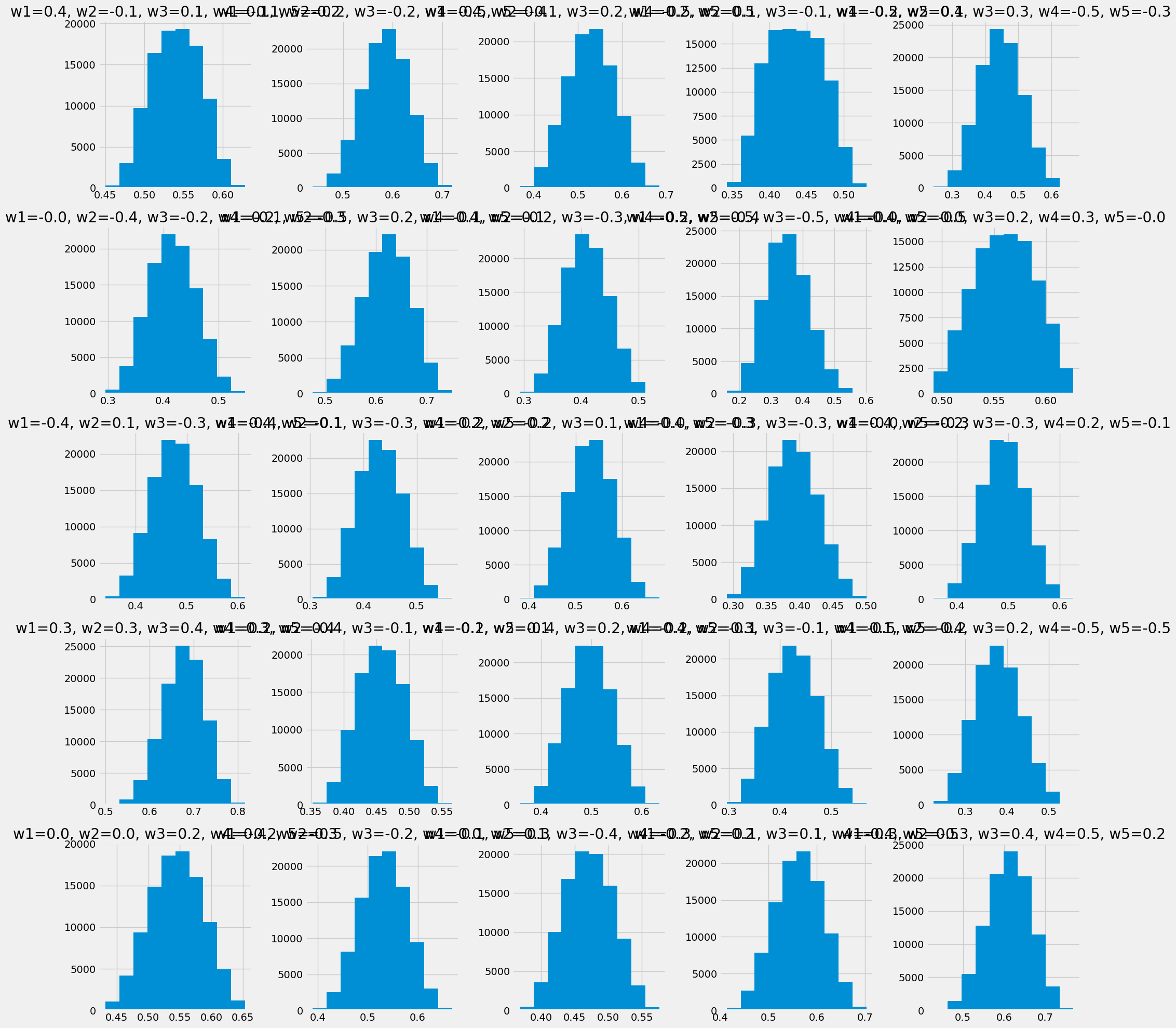


      • hmm, can't say these distributions are looking that much wider actually.
    • Ok then this constraint is just a reality then. Then maybe as far as using this for classification purposes, this should be scaled to (0, 1) maybe?