Here I’m doing one of the Keras hello world micro projects, involving classification of tiny 28x28 wardrobe images. This was really fun. ( Here’s the original home for the python notebook). One really fun part of this was that at the end I hand drew my own clothing samples, paired them down using the python PIL library and threw them against the classifier. Surprisingly, the mini model performed really well. That’s some generalizability!
Also this was a really nice expansion of my existing matplotlib knowledge. The grid plotting protips here were a great addition to my repertoire.
from __future__ import absolute_import, division, print_function, unicode_literals

# TensorFlow and tf.keras
import tensorflow as tf
from tensorflow import keras

# Helper libraries
import numpy as np
import matplotlib.pyplot as plt

print(tf.__version__)
1.13.1
fashion_mnist = keras.datasets.fashion_mnist

(train_images, train_labels), (test_images, test_labels) = fashion_mnist.load_data()
Downloading data from https://storage.googleapis.com/tensorflow/tf-keras-datasets/train-labels-idx1-ubyte.gz
32768/29515 [=================================] - 0s 0us/step
Downloading data from https://storage.googleapis.com/tensorflow/tf-keras-datasets/train-images-idx3-ubyte.gz
26427392/26421880 [==============================] - 2s 0us/step
Downloading data from https://storage.googleapis.com/tensorflow/tf-keras-datasets/t10k-labels-idx1-ubyte.gz
8192/5148 [===============================================] - 0s 0us/step
Downloading data from https://storage.googleapis.com/tensorflow/tf-keras-datasets/t10k-images-idx3-ubyte.gz
4423680/4422102 [==============================] - 0s 0us/step
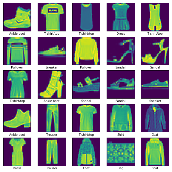
class_names = ['T-shirt/top', 'Trouser', 'Pullover', 'Dress', 'Coat',
               'Sandal', 'Shirt', 'Sneaker', 'Bag', 'Ankle boot']
plt.figure()
plt.imshow(train_images[3])
plt.colorbar()
plt.grid(False)
plt.show()
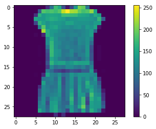
# Hmm so this `cmap=plt.cm.binary` kwarg displays grayscale instead of that strange purple to yellow scale.
plt.figure()
plt.imshow(train_images[3]/255.0, cmap=plt.cm.binary)
plt.colorbar()
plt.grid(False)
plt.show()
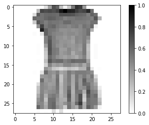
# This is almost like the output of a TSA luggage xray scanner

plt.figure(figsize=(10,10))
for i in range(25):
    plt.subplot(5,5,i+1)
    plt.xticks([])
    plt.yticks([])
    plt.grid(False)
    plt.imshow(train_images[i]) # , cmap=plt.cm.binary
    plt.xlabel(class_names[train_labels[i]])
plt.show()
train_images_scaled = train_images / 255.0
test_images_scaled = test_images / 255.0
model = keras.Sequential([
    keras.layers.Flatten(input_shape=(28, 28)),
    keras.layers.Dense(128, activation=tf.nn.relu),
    keras.layers.Dense(10, activation=tf.nn.softmax)
])
WARNING:tensorflow:From /usr/local/miniconda3/envs/pandars3/lib/python3.7/site-packages/tensorflow/python/ops/resource_variable_ops.py:435: colocate_with (from tensorflow.python.framework.ops) is deprecated and will be removed in a future version.
Instructions for updating:
Colocations handled automatically by placer.
model.compile(optimizer='adam',
              loss='sparse_categorical_crossentropy',
              metrics=['accuracy'])
# Looking at the use of the non-scaled data first.
# Wow that looks like terrible accuracy.
model.fit(train_images, train_labels, epochs=5)
Epoch 1/5
60000/60000 [==============================] - 4s 70us/sample - loss: 14.5146 - acc: 0.0995
Epoch 2/5
60000/60000 [==============================] - 4s 66us/sample - loss: 13.7328 - acc: 0.1479
Epoch 3/5
60000/60000 [==============================] - 4s 66us/sample - loss: 13.0450 - acc: 0.1906
Epoch 4/5
60000/60000 [==============================] - 4s 66us/sample - loss: 13.0474 - acc: 0.1905
Epoch 5/5
60000/60000 [==============================] - 4s 68us/sample - loss: 12.9979 - acc: 0.1936


<tensorflow.python.keras.callbacks.History at 0x139540978>
# Yea if that is out of 1.0 then this 0.1917 is pretty low
test_loss, test_acc = model.evaluate(test_images, test_labels)

print('Test accuracy:', test_acc)
10000/10000 [==============================] - 0s 26us/sample - loss: 13.0283 - acc: 0.1917
Test accuracy: 0.1917
# Try on that scaled data now ..
# Okay this looks better. more like the result in the tutorial.
model.fit(train_images_scaled, train_labels, epochs=5)
Epoch 1/5
60000/60000 [==============================] - 4s 68us/sample - loss: 0.5902 - acc: 0.8182
Epoch 2/5
60000/60000 [==============================] - 4s 66us/sample - loss: 0.3900 - acc: 0.8622
Epoch 3/5
60000/60000 [==============================] - 4s 67us/sample - loss: 0.3526 - acc: 0.8739
Epoch 4/5
60000/60000 [==============================] - 4s 66us/sample - loss: 0.3319 - acc: 0.8788
Epoch 5/5
60000/60000 [==============================] - 4s 66us/sample - loss: 0.3141 - acc: 0.8858


<tensorflow.python.keras.callbacks.History at 0x1424e8fd0>
model.input_shape, model.output_shape
((None, 28, 28), (None, 10))
model.weights
[<tf.Variable 'dense/kernel:0' shape=(784, 128) dtype=float32>,
 <tf.Variable 'dense/bias:0' shape=(128,) dtype=float32>,
 <tf.Variable 'dense_1/kernel:0' shape=(128, 10) dtype=float32>,
 <tf.Variable 'dense_1/bias:0' shape=(10,) dtype=float32>]
test_loss, test_acc = model.evaluate(test_images_scaled, test_labels)

print('Test accuracy:', test_acc)
10000/10000 [==============================] - 0s 34us/sample - loss: 0.3489 - acc: 0.8740
Test accuracy: 0.874
predictions = model.predict(test_images_scaled)
predictions[0], test_labels[0]
(array([1.3787793e-05, 5.9650089e-09, 1.9482790e-07, 1.8630770e-09,
        3.6141572e-07, 3.6579393e-02, 1.0138750e-05, 1.5758899e-01,
        1.9775856e-04, 8.0560941e-01], dtype=float32), 9)
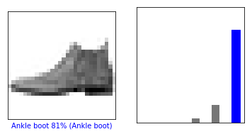
def plot_image(i, predictions_array, true_label, img):
  predictions_array, true_label, img = predictions_array[i], true_label[i], img[i]
  plt.grid(False)
  plt.xticks([])
  plt.yticks([])

  plt.imshow(img, cmap=plt.cm.binary)

  predicted_label = np.argmax(predictions_array)
  if predicted_label == true_label:
    color = 'blue'
  else:
    color = 'red'

  plt.xlabel("{} {:2.0f}% ({})".format(class_names[predicted_label],
                                100*np.max(predictions_array),
                                class_names[true_label]),
                                color=color)

def plot_value_array(i, predictions_array, true_label):
  predictions_array, true_label = predictions_array[i], true_label[i]
  plt.grid(False)
  plt.xticks([])
  plt.yticks([])
  thisplot = plt.bar(range(10), predictions_array, color="#777777")
  plt.ylim([0, 1])
  predicted_label = np.argmax(predictions_array)

  thisplot[predicted_label].set_color('red')
  thisplot[true_label].set_color('blue')
i = 0
plt.figure(figsize=(6,3))
plt.subplot(1,2,1)
plot_image(i, predictions, test_labels, test_images)
plt.subplot(1,2,2)
plot_value_array(i, predictions,  test_labels)
plt.show()
thisplot = plt.bar(range(5), [.1, .2, .3, .4, .9], color="#777777")
thisplot[2].set_color('orange')
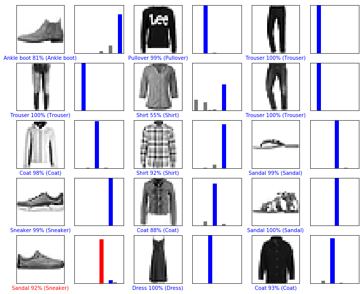
# Plot the first X test images, their predicted label, and the true label
# Color correct predictions in blue, incorrect predictions in red
num_rows = 5
num_cols = 3
num_images = num_rows*num_cols
plt.figure(figsize=(2*2*num_cols, 2*num_rows))
for i in range(num_images):
  plt.subplot(num_rows, 2*num_cols, 2*i+1)
  plot_image(i, predictions, test_labels, test_images)
  plt.subplot(num_rows, 2*num_cols, 2*i+2)
  plot_value_array(i, predictions, test_labels)
plt.show()
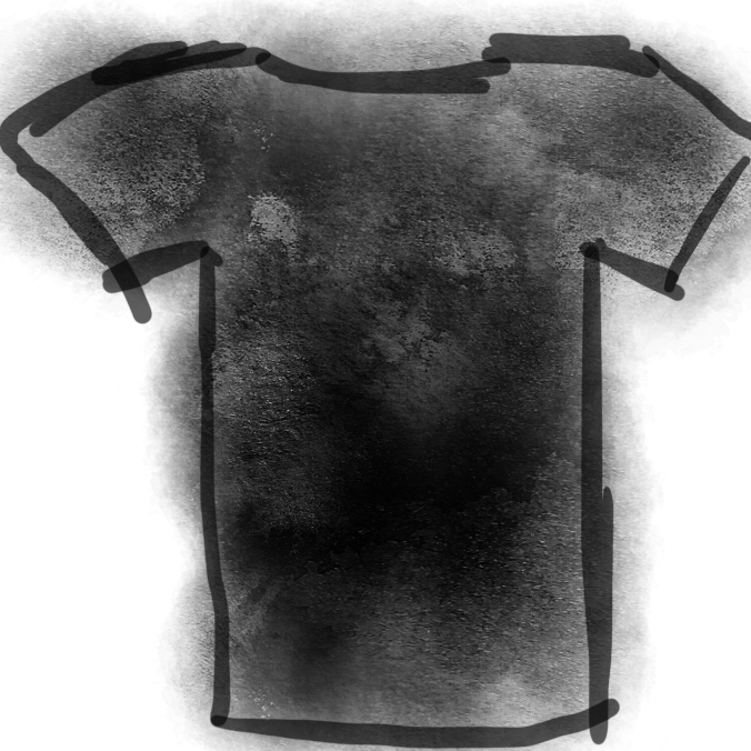
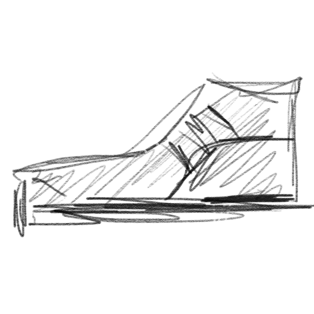
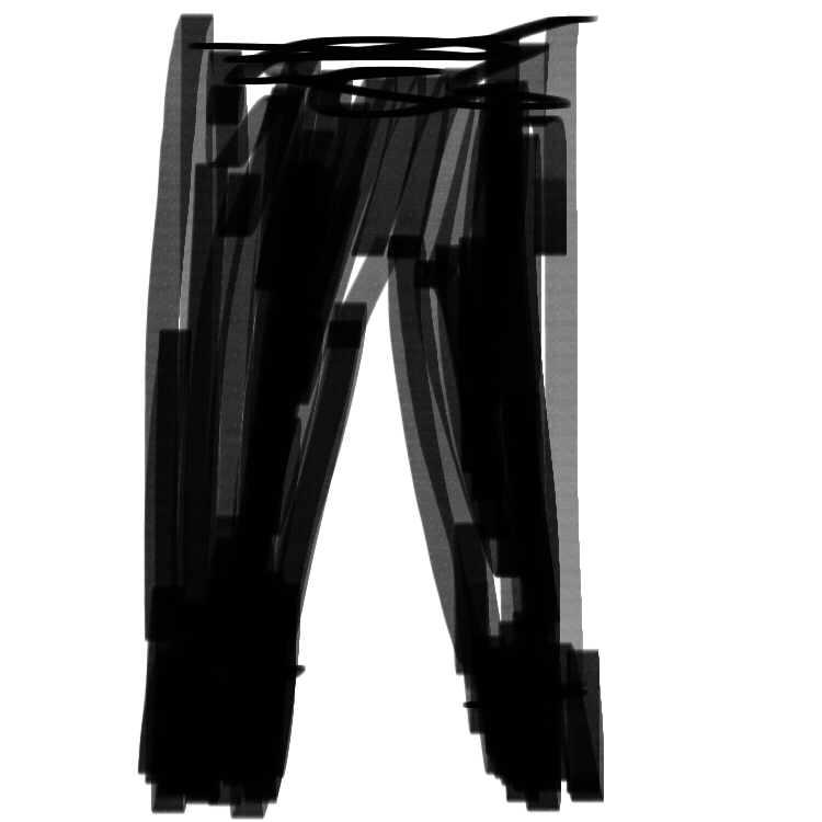
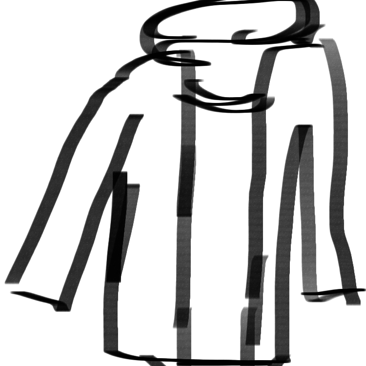
# For fun, I want to try and run the model on my own hand drawn images.
# Raw im
import IPython.display as ipd # import Image

# These four pngs were created w/ Adobe sketchbook
# Then I manually cropped them with macOS Preview to make sure they are squares.
rawnames = ['2019-05-13 14.29.04.png',
                 '2019-05-13 14.30.20.png',
                 '2019-05-13 14.31.18.png',
                 '2019-05-13 14.32.27.png']
filenames = [
        'keras-fashion-helloworld/myimages-originals/' + x
        for x in rawnames
    ]

[ipd.display(ipd.Image(filename=fn))
    for fn in filenames]
# ipd.Image(filename='keras-fashion-helloworld/myimages-originals/2019-05-13 14.29.04--8.png')
[None, None, None, None]
# with the help of PIL, obtained with `pip install Pillow`
from PIL import Image

def extract_vec(img):
    # re-scale to 28x28 in place
    img.thumbnail((28, 28), Image.ANTIALIAS)

    values = list(img.getdata())

    pixels = np.array([x[0] for x in values])

    return np.resize(pixels, (28, 28))
# quick example of first image,
print(extract_vec(Image.open(filenames[0])))
[[254 250 240 238 242 255 255 252 247 232 226 226 228 229 228 229 228 234
  244 246 245 247 248 255 255 254 255 255]
 [244 223 195 187 170 143 137 141 139 155 172 171 185 194 190 186 183 189
  121 101 110 113 104 147 205 242 249 255]
 [226 195 148  86  26  13  29  52  65  78  71  89 103 114 115 104  92  74
   61  99 103  99  82  58  67 148 224 248]
 [202 117  52  47  53  61  86  88  91  96  91  84  79  79  75  74  78  71
  111 120 122 129 115  99  94  79 109 218]
 [104  59  84  97  67  56  54  50  65  68  72  82  89  94  93  97 115 109
  125 115  92  94  82  69  70  89  89 112]
 [ 89 139 127  79  58  53  61  48  55  63  52  51  59  63  64  69  79  86
  110 119  91  75  79  71  69  72 110 138]
 [159  77 115 106  76  68  74  57  53  55  40  41  52  58  57  60  65  68
   88 101  97 100  92  84  94  98 107 117]
 [213 149  62 100  97  76  70  58  61  84  80  43  56  67  62  53  60  55
   57  70  94 108 107 112 107 119  90 148]
 [216 198 126  43 102 100  62  69  84  88 102  59  57  68  58  55  64  66
   64  61  88  98 104 137 131  99 115 179]
 [248 226 208 110  61  62  47  55  86  69  55  57  64  67  57  49  67  82
   76  66  87  87  67 106 129 108 169 199]
 [255 254 249 214  51  89 159  94  69  57  43  45  58  53  37  33  44  48
   51  50  68  74 125 158  71 130 212 231]
 [255 255 255 255 212 165 223  91  51  45  42  39  40  39  45  47  37  41
   42  41  58  63 136 235 209 200 236 252]
 [255 255 255 255 255 242 189  69  53  59  52  37  27  35  58  59  47  45
   36  34  55  60 139 237 242 248 252 254]
 [255 255 255 254 254 247 157  61  71  76  60  33  26  27  42  55  58  45
   36  32  55  62 130 245 252 254 254 255]
 [255 255 255 254 255 237 154  67  79  64  46  28  16  18  36  52  48  36
   29  37  58  56 114 240 255 254 255 255]
 [255 255 255 254 255 245 162  67  62  52  40  24  12  11  24  36  33  23
   25  32  52  58 113 232 255 255 255 255]
 [255 255 255 255 255 249 185  70  47  37  33  30  20  12  12  19  17  13
   17  23  50  56 106 227 254 255 255 255]
 [255 255 255 255 255 252 192  77  49  38  33  31  18   9   6  10  12   9
   11  22  56  52  98 219 250 255 255 255]
 [255 255 255 255 255 254 212  86  53  38  38  34  14   5   5   8   7   7
   14  25  59  58  77 209 247 255 255 255]
 [255 255 255 255 254 255 248 119  35  23  24  21  11   5   6  10  10  11
   16  35  72  69  62 205 251 255 255 255]
 [255 255 255 255 255 253 255 155  37  23  10   9   7   6  12  17  14  12
   20  45  73  65  67 205 251 255 255 255]
 [255 255 255 255 255 254 255 155  53  43  25  23  19  17  23  27  19  20
   27  47  76  78  73 208 252 255 255 255]
 [255 255 255 255 254 255 245 152  73  64  33  29  28  31  44  43  33  36
   43  57  78  89  75 216 254 255 255 255]
 [255 255 255 255 255 255 239 155  68  76  41  26  25  45  62  63  49  51
   63  76  92  97  79 211 252 255 255 255]
 [255 255 255 255 255 255 239 159  69  75  55  32  36  57  69  72  64  63
   82  94 114 116  99 223 251 255 255 255]
 [255 255 255 255 255 255 240 165  89 103  71  52  60  74  75  76  80  88
  124 134 134 143 114 233 252 255 255 255]
 [255 255 255 255 255 255 253 184  85 107  82  68  74  93  94  91  93 109
  149 163 137 102  79 239 255 254 255 255]
 [255 255 255 255 255 255 255 235 175 138 106  93  84  81  78  71  71  75
   91 102 125 155 175 255 254 255 255 255]]
filenames[0]
'keras-fashion-helloworld/myimages-originals/2019-05-13 14.29.04.png'
#
my_clothing_vecs = np.array([extract_vec(Image.open(fn)) for fn in filenames])

# and so lets try and display them with matplot lib again like the provided images...
plt.figure(figsize=(10,10))
for i in range(len(my_clothing_vecs)):
    plt.subplot(2, 2, i+1)
    plt.xticks([])
    plt.yticks([])
    plt.grid(False)
    plt.imshow(my_clothing_vecs[i]) # , cmap=plt.cm.binary
    plt.xlabel(rawnames[i])
plt.show()
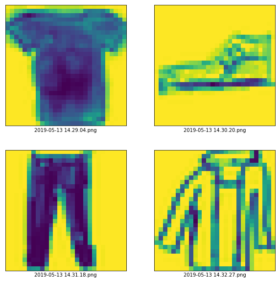
my_clothing_vecs.shape
(4, 28, 28)
# Ah crap, this looks inverted compared to what I see in the tutorial.
# Going to attempt to invert that real quick...

invert255 = lambda x: abs(255 - x)

def invert_many(img_vec):
    input_shape = img_vec.shape
    length = input_shape[0] * input_shape[1]

    invert_pxl = lambda x: abs(255 - x)

    return np.resize(
        [invert_pxl(x)
         for x in np.resize(img_vec, (1, length))],

                     input_shape)
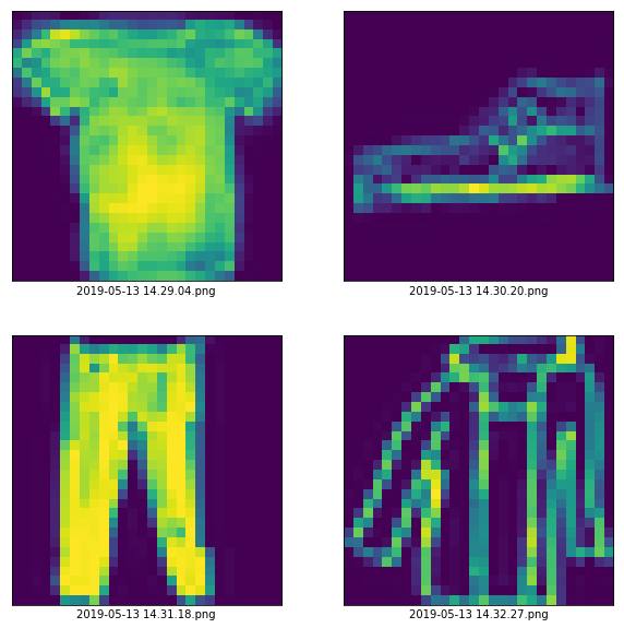
# invert them all
clothing_vecs_inverted = np.vectorize(invert255)(my_clothing_vecs)
my_clothing_vecs.shape, clothing_vecs_inverted.shape
((4, 28, 28), (4, 28, 28))
# Okay cool... now this looks like the other earlier data.

plt.figure(figsize=(10,10))
for i in range(len(clothing_vecs_inverted)):
    plt.subplot(2, 2, i+1)
    plt.xticks([])
    plt.yticks([])
    plt.grid(False)
    plt.imshow(clothing_vecs_inverted[i]) # , cmap=plt.cm.binary
    plt.xlabel(rawnames[i])
plt.show()
# Now lets see what the predictions say

# First the scaling...
my_scaled_and_inverted = clothing_vecs_inverted/255.0

newpredictions = model.predict(my_scaled_and_inverted)
print(list(enumerate(class_names)))
[(0, 'T-shirt/top'), (1, 'Trouser'), (2, 'Pullover'), (3, 'Dress'), (4, 'Coat'), (5, 'Sandal'), (6, 'Shirt'), (7, 'Sneaker'), (8, 'Bag'), (9, 'Ankle boot')]
my_test_labels = np.array([0, 7, 1, 4])
newpredictions
array([[4.26309437e-01, 2.92650770e-06, 1.60550058e-04, 9.47394001e-04,
        1.30431754e-05, 1.05808425e-07, 5.70735812e-01, 5.16380161e-10,
        1.83065375e-03, 7.26391747e-09],
       [2.88550858e-03, 3.26211921e-05, 8.07017728e-04, 7.98632973e-05,
        3.09603085e-04, 7.77611732e-01, 1.04915572e-03, 1.50996149e-01,
        6.37709629e-03, 5.98511957e-02],
       [1.78965013e-02, 8.74079406e-01, 4.85132486e-02, 3.52283381e-03,
        3.91321108e-02, 1.26371131e-04, 1.65334735e-02, 1.32581690e-07,
        1.95919056e-04, 2.40851268e-08],
       [6.74940348e-02, 6.74244831e-04, 7.51323474e-04, 2.22629853e-04,
        3.27958390e-02, 3.78045649e-03, 6.39505684e-01, 7.55926128e-04,
        1.57964438e-01, 9.60554630e-02]], dtype=float32)
# Plot the first X test images, their predicted label, and the true label
# Color correct predictions in blue, incorrect predictions in red
num_rows = 2
num_cols = 2
num_images = num_rows*num_cols
plt.figure(figsize=(2*2*num_cols, 2*num_rows))
for i in range(num_images):
  plt.subplot(num_rows, 2*num_cols, 2*i+1)
  plot_image(i, newpredictions, my_test_labels, my_scaled_and_inverted)
  plt.subplot(num_rows, 2*num_cols, 2*i+2)
  plot_value_array(i, newpredictions, my_test_labels)
plt.show()
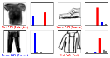
# Wow, that looks pretty good.
# - Haha apparently the Tshirt I drew looks a bit more like a "Shirt"
# - And my coat looks like a "Shirt" . Of course that was expected. I have no idea how that distinction
#     is captured by the model
# - And yea, my sneaker looks kind of like a sandal? Okay makes sense.